
By Matan Rabi and Scott Nyberg.
Salesforce Einstein’s data scales generate terabytes of data each day to train, test, and observe AI models. By only utilizing one machine, this time-consuming process could take days or weeks to complete.
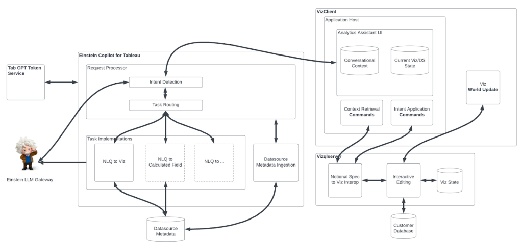
In response, Einstein’s Machine Learning Observability Platform (MLOP) team uses Apache Spark, an open-source framework module for rapid large-scale data processing. Spark enables MLOP to perform distributed computations across multiple computation units (processor cores) given a set of resources, ranging from a Kubernetes cluster to VM clusters and more.
Some of the computations and transformations MLOP team needs to do, include splitting a dataset into groups and:
- Adding a value for each row in each group. The value depends on other rows in the same group.
- Selecting the last/first/Nth row in each group. In this case, the group order has a meaning.
Apache Spark’s SQL Module has a windowing feature that allows MLOP (and you!) to achieve those goals with less code and better performance.
Read on to learn more about the added benefits of windowing and how to use them with practical use case examples.
Adding a value for each row in each group within a table
Consider this fictional transactions dataset:
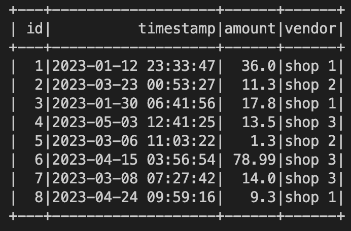
Imagine you are adding a value to each transaction, which represents the percentage of the transaction amount out of the total transactions done in the same vendor. So in this case, our group would be transactions that has the same vendor.
To address this use case without windowing, you would need to:
- Group by vendor, sum the amount, and insert it into a separate dataframe.
- Join the vendor column in the original dataframe with a newly aggregated dataframe.
- Add a new column for the transaction amount (the original dataframe) / total vendor transaction amount (aggregated dataframe).
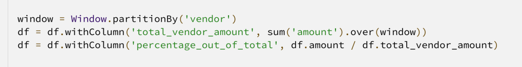
Let’s see how it looks in code:

Now, let’s examine what would have happen if you use windowing.
There are two stages to windowing:
- Creating the window. This basically represents how you want each group to appear within the table.
You can use the partition by here clause if you want to divide your groups by a key, or order by if you want to create and order your group. Note that if you use order by, the entire table will be one group. - Applying a window function over the window. You want to apply this for a row in each group. This includes aggregate functions (i.e. min, max, count, sum, avg), ranking functions (i.e. rank, ntile), and analytic functions (i.e. first_value, last_value, nth_value, lag, lead). Ranking functions and analytic functions are usually effective when you order your group(s).
Got all that? Now, the steps to achieve your above use case with windowing would be:
- Create a window partitioned by vendor.
- Apply a sum on amount over the window.
- Divide the amount with sum on amount.
Let’s see how it looks in code:
In both approaches, you’ve reached the same outcome:

By using windowing, you saved a join, did not create another dataset, and, as a special bonus, made your code neater. Of course this represents a tiny dataset, but you could imagine that for large datasets there could be a big difference in performance and efficiency.
Select the first/last/Nth row in each group within a table
This example spotlights the need to obtain the highest transaction amount for each vendor. In that case, we need to order each group (transactions that has the same vendor) by amount and select the first transaction.
If you wanted to achieve it without windowing, your steps would be:
- Group by vendor and select the max amount.
- Join the two tables, where vendor and transaction amount equals the max amount.
Your code would look like this:

Similar to the first use case, in this approach you have created an additional dataframe. Additionally, you used a join to get the wanted result.
Conversely, let’s examine the steps needed to achieve this while using windowing:
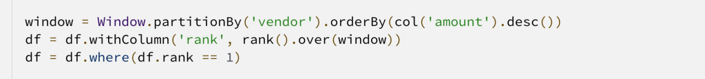
- Create a window partitioned on vendor, ordered by amount descending.
- Apply rank over the ordered window.
- Filter where rank equals to 1.
Let’s see how it looks in code:
Both would result in a similar dataframe while achieving the needed result:

But, using windowing allowed you to avoid an unnecessary join, an additional dataframe creation, and a group by. In looking at the steps (aka “verbal algorithm”) for each approach, you will see that windowing allows you to also write a more intuitive code.
MLOP’s use case for windowing
Salesforce’s MLOP team is responsible for machine learning models observability. This involves comparing the predictions made for customers vs the ground truth. In this manner, the team uses mathematical formulas to see where models excel and where they must improve.
MLOP also segments the data to pinpoint any issues. For example, a model might be performing well on Caucasian men, aged 18-25 from Indiana but underperforms on Asian women, aged 26-35 from California.
When does MLOP use windowing? It’s usually when the team uses the ground truth, which could rely on user input that might change over time, such as predicting the priority of a case. In fact, for each case ID, there could be multiple “ground truths” over time. Ultimately, for each case ID, MLOP takes the most updated ground truth.
This traces back to the above second use case: In the ground truth table, we partitioned on case ID, ordered by event timestamp, applied rank window function and filtered for rows where rank == 1.
Learn more
- Hungry for more AI stories? Check out this blog for a behind the scenes look at the MLOP team.
- To learn more about Apache Spark and how to optimize your spark applications by understanding the concept of partitions, read this blog.
- Stay connected — join our Talent Community!
- Check out our Technology and Product teams to learn how you can get involved.