At Salesforce infrastructure we are working to deploy our machine learning driven performance improvement framework to enhance customer experience globally. As with any ML solution, data is key! In order to have meaningful results, we have to consider millions of data points. This introduces a whole set of challenges, but mainly the need for a reliable source of bulk data. Generating our own synthetic data mitigates this problem by giving us the ability to test out ML algorithms in a lab environment.
While we are not simulating a network, we can simulate data samples by modeling an existing network. We can use samples from historical data to create a model that we can query for more data points as we need them.
There are a couple of reasons that drive the need to generate synthetic data rather than use live traffic:
- The synthetic data should ideally be independent and isolated from the production environment.
- Synthetic data can be generated on demand and in any quantity.
- Synthetic data gives us the ability to set specific scenarios to test our ML framework on.
- Our models give us flexibility that real data cannot provide, while still keeping true to real network behavior.
Ideally, we want to find a way to simulate the network behavior by having an insight into how the real network behaves.
Approach
Using historical data, we can fit a probability distribution that best describes the data. We can then sample the probability distribution and generate as many data points as needed for our use.
Using MLE (Maximum Likelihood Estimation) we can fit a given probability distribution to the data, and then give it a “goodness of fit” score using K-L Divergence (Kullback–Leibler Divergence). We can then choose the probability distribution with the best score as the probability distribution that best describes the data with the sufficient statistics generated using the MLE process. This process can be later used on live traffic too, improving the accuracy of the results.
Implementation
Our solution is divided into two independent stages, Data Fetching and Modeling. This is done so that, in the future, the modeling stage could be applied to any source of data.
Data Fetching
Historical data is currently pulled from a data archive that is defined by customer id and date range. The data is then decoded and filtered to include only relevant information. Metrics from the data are stored in a PostgreSQL database for subsequent modeling.
Modeled metrics are:
- access round trip time
- time to first byte
- download time
- size
- time between network requests
- link capacity
- upper and lower bound for each metric
Data Modeling
Modeling is done by fetching all the data points available for the specified scope, defined by customer id and time window. The data is then divided by geographical locations and then sub divided by networks. The data is then randomly sampled to get N samples for each sub group (usually 5000 samples). These samples are then used for fitting some of the available probability distributions in the Python library scipy.stats.
Each distribution is then given a score which is a linear combination of 3 elements (lower is better):
- K-L divergence score, which measures how close the fitted model is to the data.
- Probability of sampling numbers below the modeled lower bound.
- Probability of sampling numbers over the modeled upper bound.

Results
Each scope (geographical location + network) is assigned a probability distribution as well as its sufficient statistic together with modeled upper and lower bounds. This is then exported as a JSON file, and can be used as a configuration file when sampling from the modeled probability distributions.
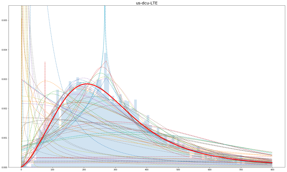


As we can see from the results, this method is quite effective in modeling metrics that are independent of other metrics, however, it can be used for dependent metrics with some post processing. With some changes, it can be upgraded to model more complicated probability distributions if a more accurate model is needed, but usually, it is good enough. It is also not limited to this specific application, rather it can be used to model many other sources of data.
Do you have other uses for synthetic data modeling? Let us know in the comments.
Follow us on Twitter: @SalesforceEng
Want to work with us? Salesforce Eng Jobs