
The AIOps team in Salesforce started developing an anomaly detection system using the large amount of telemetry data collected from thousands of servers. The goal of this project was to enable proactive incident detection and bring down the mean time to detect (MTTD) and mean time to remediate (MTTR)
Simple problem, right?
Our solution was to create a forecasting model with the time-series observability data to predict the potential spikes or dips causing incidents in various system and application metrics.
Let’s take a deep dive and validate our hypothesis.
We decided to start with a univariate approach on a single metric which represents the average page load time for our customers.
How many models do we need? Answering this question isn’t simple.
1 time-series metric = 1 model
Too easy? Unfortunately the real world is a difficult one.
The inbound traffic pattern and seasonality is completely different for various regions (Asia Pacific/North America/Europe etc). We have to factor in this variable to generate good predictions.
10 Regions x 1 time-series metric = 10 models
Are we sure that each datacenter serving a region has the same type of hardware specification?
Not at all. Based on the procurement period, we keep updating the hardware specification. So, it’s good to have host level models.
10 Regions x ~10k hosts x 1 time-series metric = 100k models
Are we done yet? Here comes the interesting part.
Let’s say we collect the metric in a minute interval and use that for training the model. Using the lowest granularity available is very important to find minor service degradations, but the downside of this approach is noisy alerts. Alerts caused by minor glitches are normally not actionable and do not cause any customer impact. One way to generate quality alerts from time-series data is to create an ensemble of models trained on data aggregated at different time intervals.

We generated models for the metric with data aggregated over 1 minute, 15 minutes, and 1 hour. The higher the interval, the higher the weightage we give to the models. A spike on data averaged at a minute level may not be an incident, but the same spike on data averaged at an hourly level can cause a serious incident.
Let’s count the number of models again:
10 Regions x 10k hosts x 1 time-series metric x Ensemble of 3 models = 300k models
Now you can see that, starting from 1 model, we are about to produce 300k models. But its not 1 million yet, right? This is rough math for a univariate approach. Designing a proactive incident detection system uses a lot of system and application metrics. Once we add multiple metrics to the system, the final number would be the number of metrics times 300k.
Serving models (fast)
Now that we have time-series models with very high accuracy, the next challenge is model serving. It is of no use if we can’t serve these models fast for real-time data. We have a couple of options here: use one of the open source platforms, or build one ourselves. As a first step, we evaluated MLflow and Kubeflow. (There are many other open source products, but we decided to evaluate the most popular ones first.) Both of these platforms offer solid model serving options with a lot of features. But these projects were in very early stages with a lot of changes going in when we started this project in early 2019, so we decided to park these options and started to work on building an easy way to serve models. Simple and fast is what we needed, not a lot of features.
The first thing was to come up with an abstraction of prediction for models generated by various libraries.
class Model(abc.ABC):

    def predict(self, model_id, data_points):
    """
    Predicts anomaly scores for time series data
    """
We implemented predict for all distinct kinds of models that we use. Models are generated with various open source libraries and custom algorithms developed internally.
The last step is to invoke the predict method from a simple web app. We used Flask. You can see the sample code below.
import pandas as pd

@app.route('/predict', methods=['POST'])
def predict():
    """
    Predicts anomaly score for time-series data
    """
    request_df = pd.DataFrame(requests.json["datapoints"])
    model = Model(requests.json.get("model_id", default_model))
    prediction_df = model.predict(request_df)
    return jsonify({'anomaly_scores: prediction_df.to_dict('list')})
This simple code snippet can serve models. But we need to optimise the response latency to enable smooth predictions for real-time data. Let’s see how we do that.
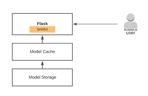
Compressing the models and adding a caching layer was important. Fetching models from storage was slow, as some of the models are large in size. Compressing models helped to reduce the storage size and network throughput more than 6x. We were able to serve ~1 million+ models generated out of 10–15 time-series metrics smoothly with this simple system.
This blog content is based on our experience and learnings from building an anomaly detection system. There are multiple ways of achieving this. You can factor in each variable as features and train a single model to serve this purpose, but the quality of alerts produced by this approach worked much better for us.