I am a Principal Engineer at Salesforce where I architect, design, and build big data systems.
Metrics Discovery is a feature that helps you find the metric names that you want to view, chart, or create alerts on. It also helps you browse the metric names that exist in the system. When you have over a billion metrics and tags, discovering them is an enormous challenge. How do we search which metric to chart from an ocean of a billion entries? How do we search them faster without hurting user experience? How do we return the metric that is most relevant to the user’s search? How do we make the discovery service reliable in the event of a network partition, or hardware failure? These are some of the problems we were trying to find solutions for. Over the past few months we made significant changes to our Argus open source project and found answers to these problems. This blog is the story of that journey.
At Salesforce we run one of the worlds’ largest time series monitoring systems supported via our open source Argus project. We ingest hundreds of billions of data points per day. On the backend we use the open source Opentsdb and Apache HBase systems to store our metrics. Apache HBase is our definitive source of truth for metric metadata. We used this backend to meet all your metric discovery needs. Our initial architecture looked like this:

But we soon outgrew our Opentsdb/HBase system for metric discovery. Discovering metrics was taking more and more time. Also, the Opentsdb/HBase-based index only supported prefix-based searches and we needed a rich search capability, so we introduced Elasticsearch to store metric metadata. We added another set of Apache Kafka consumers called schema consumers which consumed the same metrics Kafka topics and inserted the metadata about them in an Elasticsearch index. Our architecture evolved to:

This change significantly improved metric discovery speed. But maybe you can guess what happened next. Oh yes. We also outgrew this architecture thanks to volume growth. Now we had billions of tags in our single Elasticsearch index. Because of this huge volume we had a variety of challenges:
- Kafka lag for schema consumers took a very long time to catch up on a restart.
- Upgrades of schema consumers took a very long time (days).
- Schema consumers went on long garbage cleaning cycles, halting consumption
- We had 25 schema consumers consuming the Kafka topics. We could only restart one at a time, wait a few hours for it come to steady state, and then move on to the next one.
- Metric discovery performance degraded each day as our volume grew.
We went back to the code, architecture, and Elasticsearch installation to find the root cause of the above problems. And, voila, we found significant opportunities to make things better. Below is the chronological sequence of changes we made.
Robust Elasticsearch for high scale time series
- Dedicated volume for storing indices: We found that the index storage was using the same partition as the system so we separated out the Elasticsearch storage path. This gave us a larger, dedicated partition and protection against the disk getting full from other services on the node.
- Single directory for es.path.data: We were using two different directory paths that were mounted to two different disks. Elasticsearch lets you specify that path, but the side effect was that there was an uneven distribution of shards. Some nodes were getting more shards than others and causing hot-spotting. Once we switched to a single directory path, this problem went away
- Replica count: We switched from a count of 2 to a count of 3. This gave us a little more protection against hardware failure and also slightly increased our read performance.
Introduce Time in metadata index
Our Elasticsearch index contained billions of documents. We didn’t know which document arrived when. The very first thing we did was add an mts (modified time stamp) field to each document that was going into Elasticsearch. This enabled us to retire tags that hadn’t been used in the past ’N’ days. In time series monitoring, the most recent data has high value. 99% of our metrics queries were over the past 30 days. It didn’t make sense to keep the tags any longer than that in our discovery service. By the time we let this code hydrate, we had 25% more documents. We retired billions of documents in one shot once our ’N’ days had passed. We added a nightly job that would back up stale tags (older than N days) into a backup index and then delete them from the primary index. We also closed the backup index so that we could save on heap memory. If customers wanted to restore stale tags, we provided a tool to restore the stale tags from the backup index into our primary index. Elasticsearch provides a fantastic API to do this. Now, we are protected against unbounded growth. As soon as we did our first big purge, our discovery service saw a 2200% speed improvement!
Bloom Filters for Big Data
In a time series, 99% of the volume appearing on the Kafka topics has metric names that are repeated. Reading each time series data point and writing the metadata about it to the discovery index isn’t practical or necessary since it just overwrites 99% of the existing documents. You would also need a very large Elasticsearch installation to handle the high IOPS. We implemented a trie in the schema consumers as our cache. We checked the existence of a metric’s metadata in the trie before writing to Elasticsearch. This was fine when we had small cardinality, but soon we couldn’t fit all of our metrics in the JVM trie. The unintended side effect of this was that our JVM started taking long garbage collection pauses, slowing down consumption. We had to keep adding more Kafka consumers to share the load, but that didn’t help either. Soon, our trie cache hit ratio was getting lower and lower, making more writes go towards Elasticsearch. This caused a heavy load on Elasticsearch write volume as well as huge version conflict resolutions since each of the 25 schema consumers were overwriting the same document. It was about time we introduced some probabilistic data structure to address this problem. After doing some experimentation with HyperLogLog, vanilla Bloom filters, and streaming Bloom filters, we settled on the vanilla Bloom filter and replaced the trie with it. Boom. This change helped us significantly.
- We fit our entire volume of repeat metrics in Bloom filter and had room to grow 20x while consuming significantly less memory than the trie.
- We reduced our consumers to 10 (from 25) and still had room to handle 5x growth.
- We can upgrade and restart our consumers at will without increasing Kafka lag or interruption in the discovery service.
- We no longer have garbage cleaning cycle pauses.
- We reduced the load on Elasticsearch, which can now take in even more new metrics
Split Elasticsearch index
We had one single index that would store scope, metricname, tagkey and tagvalues. Here is an example of these fields,
{
“scope”: “argus.jvm”,
“metric”: “file.descriptor.open”,
“tags”: {
“host”: “my-host.mycompany.com”
}}
Our unique scopes were in the tens of thousands range, metric names were in the tens of millions, and tags were in the hundreds of millions range. Any Argus user starts their metric discovery by typing the scope. We were searching for it in a sea of millions of documents, and it didn’t make sense. So we split the scope into its own index, the metric names into another index, and kept the tags in the existing index. By making this simple change we increased scope discovery speed by 4300%. We completely got rid of the spinning wheel; no more thumb twiddling while waiting for the UI to return!
Now, our architecture looks like this:


Conclusion
- Making significant changes to an existing installation is not easy. We needed to take lots of care not to break backwards compatibility or cause service interruptions while introducing performance improvements. We had to plan things thoroughly and execute them in chronological order to have enough bake in period.
- Dealing with “real big data” is hard, when you have billions of documents in your index.
- Always have a backup of things you’re deleting and working tools in place to restore them if things go awry.
- From the point when we started this initiative to now, we increased our discovery performance by a whopping 14,200%. And we’re not done yet. There are still significant changes coming to Argus to make time series discovery robust, fast, relevant, and user friendly.
All of the above changes are available in our open source Argus project. If you have any suggestions, pull requests are most welcome. If you find working on petabyte scale big data monitoring challenging, then we are hiring. Reach out via our careers page.