Activity Platform (AP) is part of our Einstein Activity Capture (EAC) and Engagement Activity Platform (EAP) eco-system. AP captures, on behalf of users, their activities and engagement data generated from the interaction between users and their leads and contacts. Upon capturing those records, they are scoped, augmented with artificial intelligence models, stored, indexed, used to trigger alerts, and eventually counted for various metrics. This is done in a processing graph composed of many pipelines performing streaming processing in a near real-time fashion.

This blog presents a simple algebraic model that helps to analyze

1. cost planning — where over-provisioning is useful, where it is not, and the return on investment from over-provisioning.
2. pipeline degradation — by externally measurable parameters to gauge the health of a pipeline and its relationship with the Service Level Agreement (SLA)

We were frequently asked about the latency of some particular processing path. We can answer that, but maybe not in the form that the interested party is looking for. AP operates a non-trivial processing graph with different storages and runtimes in it. When there is a degradation or a service disruption in any of the computation entities, some pipelines may slow down or come to a complete halt. Even if we can measure pipeline latency and arrive at an expected value with median, deviation, and 95-percentile, it is measured when the pipeline is in full health. That is when the pipeline has no degradation and no outage.

The latency may be expressed as

The expected latency has a median of X seconds and a 95-percentile of Y seconds with a standard deviation of Z seconds when the pipeline is available and operating at the expected rate.

What if the processing pipeline starts to degrade or becomes unavailable? What is the behavior of the expected latency when that happens? How long can an outage be and how soon can the system recover from it? A logical question to ask would be what the expected Availability SLA should be.

Availability vs Downtime

Downtime does not spread evenly across every single day [1]. It might happen a few times in a year. Even with a downtime of 52 minutes once a year, the pipeline still meets 99.99% availability. It is not a short time for users to wait for 52 minutes for data to show up. We want to do it better than that. But what is the cost of having a processing pipeline with north of 99.99% availability?

A typical processing pipeline is composed of a few processing runtime entities such as Apache Storm topologies, Kafka Streaming processes and Spark Streaming jobs. The processing runtimes access storage systems such as NoSQL databases, search indices, relational databases and distributed caches. In between those processing runtime entities, there are Kafka brokers as a persistent messaging storage to daisy chain the processing pipeline. Due to the nature of the asynchronous processing which relies on a queuing system with high availability, when estimating availability, we often assume the queuing system has a near 100% availability, thus discounting them for availability degradation. A typical pipeline spans 5 to 6 processing runtimes and storage clusters. A longer pipeline includes up to 11 or 12 runtimes and storage.

If 99.99% is called 4–9er availability, 99.95% is 3–9 plus,

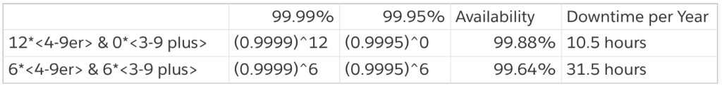
If each entity has a 4–9er availability, the pipeline’s overall availability is 99.88%. It is roughly 10.5 hours per year. If half of the runtimes or storages have only 3–9 plus availability, the pipeline’s availability dropped to 99.64%, 31.5 hours per year. It is longer than a day! It would require an all 5–9ers in such a long pipeline to make the pipeline close to being 99.99% available (0.99999¹²=0.99988). It takes extremely robust components to form a decent pipeline.

Availability and Latency

We started with a question regarding pipeline processing latency, yet spiraled into a discussion of availability. What is the relationship between latency and availability, if there is one?

It is safe to say that some perturbation in latency, say, within an order of magnitude from the 95-percentile value, is not an availability concern. However, availability affects latency dramatically. As an extreme example, when the processing pipeline is down, the processing latency of new activities is equivalent to infinity. Many things affect a pipeline’s availability, such as the pipeline’s architecture, the components of its technology stack, and the quality of software design and implementation. But they are intrinsic qualities. Once the pipeline is deployed, there are only a few operational options to safeguard availability, such as high-fidelity monitoring and capacity planning.

It was, at one point, suggested to use over-provisioning as a defense to pipeline degradation and a fast recovery mechanism after pipeline is restored from outage. While it sounds like a plausible choice, two questions arise.

1. How effective is over-provisioning as a defense to performance degradation and a recovery mechanism to outage?
2. What is the right level of investment for over-provisioning?

Scenarios and Models

We analyzed a few traffic patterns to come up with an algebraic model.

1. A complete outage period followed by a recovery period to consume accumulated backlog
2. An overall throughput degradation
3. A throughput degradation caused by partial outage of a sub-stream in a pipeline
4. Tsunami traffic
5. Continuous surface wave

A Complete Outage Followed by a Recovery Period

This is the most basic and most common scenario. A computation runtime or a storage used in the pipeline suffers an outage that stops the traffic flow through the pipeline. At the same time, a backlog of arriving data starts to build up and waits to be processed.

Say the average rate of data arrival for a pipeline is R. After an outage duration T, the backlog will be T*R. Once the pipeline is restored to health, it starts to consume the backlog at its provisioned peak rate. If the over-provision factor is N, the peak processing rate is N*R.

R : Average rate of data arrival
T : Pipeline down time
T*R : Accumulated amount of to-be-ingested data during down time, aka backlog.
N : Factor of over-provisioning. When N = 1, it means there is no excessive capacity with respect to the average rate of data input R.
N*R : Provisioned pipeline ingestion rate, or pipeline peak capacity, denoted as NR.

As the pipeline takes time to consume the backlog accumulated during the outage period, another, smaller backlog builds up. The duration it takes to consume the initial backlog is TR/NR (=T/N), and the second backlog during this time is R*(T/N). The processing pipeline needs to take extra time, [R*(T/N)]/NR, to consume this new backlog. This process continues until the new backlog becomes negligible and new data can be processed as soon as they arrive.

We denote P as the time to recovery and A as the total time of pipeline disruption.
P : Time to consume backlog, or Recovery Period or Recovery Duration
A : Total time until a pipeline returns to normal processing, or Total Time of Disruption or Total Time of Despair. A = T+P

Recovering Time

P = (TR)/(NR) + [(TR/NR)*R/NR] + {[T/(N*N)]*R/NR} + ……
P = T/N + T/(N*N) + T/(N*N*N) +……

P = T/(N-1)

Total Time of Disruption

A = T + P
A = T + T/(N-1)

A = T[N/(N-1)]

Let’s take a closer look at this result, especially the quantitative effect of outage duration T, and over-provision factor N.

Determine Acceptable Pipeline Down Time, T

Using SLA to project T is not to project the worst-case scenario, but rather to determine what is acceptable. If we assume the yearly SLA value is Ly, the outage duration T has to be no bigger than the yearly SLA value, T <= Ly. Depending on how stable the pipeline is, T may be larger than Lq, a quarter of the yearly SLA. If it only happens once or twice a year, the system can still meet the yearly SLA. This is the acceptable upper bound for outage duration T.

As we do not want to set overly sensitive alert thresholds such that false alarms may be generated, it may take 5 to 10 minutes to detect a pipeline anomaly when the pipeline stalls. It may take another 5 to 10 minutes to determine the root cause and decide on proper actions. Overall, it can take between 20 to 30 minutes, the soonest, for the pipeline to resume processing and start to burn down backlog. This is the lower bound of outage duration taken from empirical data.

From the two conditions, we can see, Z <= T <= Ly.
L — the SLA value
Ly — the yearly SLA value
Lq — the quarterly SLA value
Z — the time duration from the onset of outage to the moment pipeline regain full strength

The outage duration can only be between 20 minutes and 50 minutes if the pipeline is to meet 99.99% SLA. However, this is not the whole story, as outage duration does not include the duration from the recovery period when the pipeline’s latency still exceeds the target range.

Cost versus Benefit of Over-Provision, N

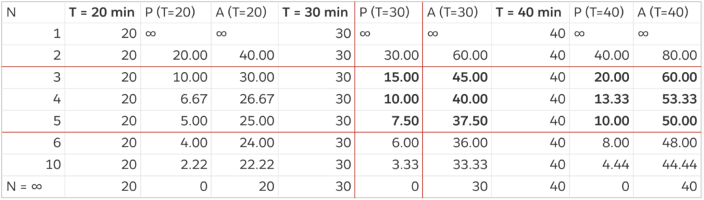
The following table demonstrates a few effects.

• If there is no over-provisioned capacity, N=1, the damage from an outage will never recover.
• The benefit of over-provisioning is on a curve of diminishing return. The benefit of increasing N from 2 to 3 is significant. As the over-provision factor gets higher, say N>6, the reduction in recovery duration may not justify the additional cost.
• We derived a condition in the previous section that the outage duration should be controlled between 20 to 50 minutes. If the recovery period is included, the outage period has to be further limited to under 40 minutes.

A diminishing return as the provisioned processing capacity increases

N : over-provision factor
T : pipeline outage duration
P : pipeline recover or catch-up duration
A : total time of pipeline disruption

There are also some not-so-obvious points in this formula that are worth noting.

• As the over-provisioning factor N increases towards fairly large (10 < N → ∞), the pipeline seems to have the ability to consume backlog instantaneously. This formula of total duration does not include pipeline restart cost. As the size of the pipeline increases, if the recovery mechanism requires restarting certain clusters in the pipeline, it will take more time for the cluster to restart as it gets bigger.
• It is relatively fast to scale up CPU, memory, and thus the total I/O of the stateless components in the pipeline, such as Storm worker hosts or Spark executors. It takes much longer to scale up storage, and the procedure can be delicate. To balance between cost and pipeline robustness, it would be advantageous to have storage provisioned at the designated over-provision factor, while keeping computation cluster smaller to save cost. This effect becomes obvious in the face of tsunami traffic.

Overall throughput degradation

Throughput degradation happens when the pipeline is processing at a fraction of ingestion rate R.

Latency is usually higher than the typical latency benchmark value when degradation happens. It often is associated with some failed workers in the processing cluster or troubled storage layer.

It is easy to spot a really bad degradation. It is hard to observe a capacity degradation when the throughput is not lower than R, the average data rate. That is for a degraded throughput dR, where d is the degradation ratio, 1 < d < N, R < dR < NR. In a lot of cases, processing latency shows early signs of warning. It gives a better indication before d drops below 1.

Recovery time

1 < d < N, there is no recovery time since there should be no real backlog.
When d < 1, let T be the duration of throughput degradation and the backlog during this time is B.
B = (1-d) * R * T
The equivalent time of pipeline stall is T’
T’ * R = (1-d) * R * T
T’ = (1-d) * T

P = T(1-d)/(N-1)
A = T(1-d)[N/(N-1)]

Sub-stream Stall or Slowness

Sometimes we see a single Kafka partition or a few partitions stall, or have severe throughput degradation. Unfortunately, other healthy sub-streams cannot share the load for the troubled sub-stream without changing traffic routing rules. The recovery time is as long as the whole pipeline experiencing the same hardship.

Sub-stream stall
P = T/(N-1)
A = T[N/(N-1)]Sub-stream throughput degradation
P = T(1-d)/(N-1)
A = T(1-d)[N/(N-1)]

For organizations having traffic flow in the affected sub-stream, the user experience is the same as if the whole pipeline is suffering the same issue. Fortunately, we do not see sub-stream stall or degradation often. When it happens, it is usually due to data skew from a few organizations. Its cause and remedy is beyond the scope of this blog and probably worth one of its own.

Tsunami Traffic

A definition of tsunami traffic is continuous incoming traffic for a prolonged duration with an arrival rate well above the over-provisioned throughput rate, and the duration may have already breached the availability SLA. When tsunami traffic hits, the pipeline is processing at its peak rate. The traffic flow does not stop, but a traffic backlog starts to grow. Since the processing does not stop, the analysis is different from that of an outage. We can tackle this in any of the following approaches to develop a benchmark for pipeline capacity investment.

1. Treat the over-provisioned capacity as a degraded capacity relative to the tsunami traffic rate
2. Use the backlog consumption model to compute the recovery time after tsunami traffic subsides
3. Calculate the delay suffered by an arbitrary data record arriving after the backlog forms

The first and second methods are identical and should be an easy exercise in applying what we have derived in the section of Overall Throughput Degradation. The issue is that we do not know the strength of the tsunami beforehand. We want to develop a model to gauge the pipeline capacity and its effectiveness with regard to various strength of the tsunami flow.

We introduce an indicator of pipeline resilience, X. X is measured as the duration that a tsunami can last before the SLA suffers. This indicator gives us a sense of “how much time we have before users start to feel the pain.” Naturally, X is a function of the total provisioned capacity of the pipeline and the strength of the tsunami.

X = ƒ(N, R, U)

U : the tsunami traffic rate
S : S = U – NR, the excess rate of tsunami traffic above over-provisioned capacity. S exists when U > NR and S > 0
X : the resilience against tsunami traffic measured in time

Analysis by Backlog consumption during recovery

This is method 2, “Use the backlog consumption model to compute the recovery time after tsunami traffic subsides”.
If the total backlog generated during tsunami is B, B equals X*S.

B = XS

P = XS/NR + [(XS/NR)*R]/NR + [XS/(NR*N)]*R/NR + ……
P = (XS/R) * [ 1/N + 1/(N*N) + 1/(N*N*N) + …… ]
P = (XS/R) * [1/(N-1)]

P = XS/[R*(N-1)]

If P ~= L, recovering time is close to availability SLA; any data coming to the processing pipeline after tsunami traffic has subsided will not be processed until after recovering time P. It is like the system was down that long and availability SLA has been breached.

L = P = (XS/R) * [1/(N-1)]
X*(S/R) = L*(N-1)

X = L * (N-1) / (S/R)
or
X/L = (N-1)/(S/R)

Note that for S to exist, the traffic has to exceed the total capacity. The higher the value NR is, the less likely for S to occur. This is be seen by the following equation.

U/R = (N-1) * L/X + N

Where U > NR, U/R > N.

Let’s demonstrate the resilience by an example.

U = 5R, that is the traffic is 5 times of the regular traffic rate.

For N = 3
S = U – NR = 2R => S/R = 2
X = L

For N = 4
S = U – NR = R => S/R = 1
X = 3L (resilience is 3 times of SLA time)

In this case, 33% more investment gives 3 times more system resilience. However, N cannot be too high due to diminishing return on recovery time for pipeline stall.

X/L: resilience indicator. The higher the ratio, the more resilient the pipeline is against huge influx of data.

Why use availability SLA when the pipeline is not down?

When the backlog is so severe, the incoming traffic is queued in the queuing storage unprocessed for an extensive period of time. For applications depending on timely processing of data, this is equivalent to the system being down.

Approximation

Tsunami traffic does not start and end like a step function as assumed in the calculation. When the traffic ramps up, the initial flood may be absorbed by the over-provisioned pipeline capacity. The above modeling gives a good approximation. However, when the traffic subsides, the calculation assumes the input rate reduces to average rate R immediately. Therefore, it tends to underestimate the recovery time. Since the model is calculated based on the assumption that recovery time is close to SLA, P ~= L, an approximation itself, the induced error is not significant as long as the strength of the tsunami traffic is not more than an order of magnitude higher than the over-provisioned pipeline capacity.

Observation

During a large traffic storm, the processing/networking/storage infrastructure is under great stress. It is important to monitor it and make sure the over-provision factor N is maintained. If we want to increase its capacity, it is probably easier and faster to increase processing workers and number of connections. But it takes longer time to ramp up storage capacity, as storage may need to perform re-distribution and replication when the cluster is expanded. If there is any single node component in the processing pipeline, such as RDS instances, it can be the component that triggers performance degradation.

Analysis by Eager Waiting Data

This is method 3: “Calculate the delay suffered by an arbitrary data record arriving after the backlog forms.”
It is analyzed is by looking at a particular message enqueued and the wait time for that message.

X * (U-NR) = N * R * L
X * S = N * R * L

X = L * N /(S/R)
or
X/L = N / (S/R)

This is a slightly optimistic definition for pipeline resilience.
Using the same example, U = 5R

For N = 3
S = U – NR = 2R => S/R = 2
X = 3L/2

For N = 4
S = U – NR = R => S/R = 1
X = 4L

Comparison of the two analyses (X/L)

In both models, the pipeline resilience against tsunami traffic increases along with the increased over-provisioning capacity. The difference between the two methods is that backlog consumption analysis observes from outside until the backlog is gone, while eager waiting analysis observes the congestion from inside the traffic. As the observation from outside presents a stricter resilience model (X/L values are smaller), it makes us feel more confident using backlog size as one of the key indicators to measure.

Continuous Surface Waves

Input traffic

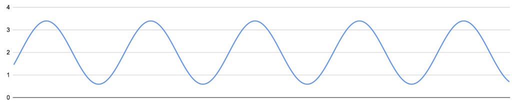
Throughput pattern

The above two diagrams illustrate an example of continuous surface waves. The average traffic rate to the pipeline is R and the total provisioned capacity is 3R. The incoming traffic has an input rate oscillates from less than R to more than 3R.

We have not developed a suitable model for this type of traffic. Intuitively, if the excessive data do not exceed the area between the two peaks, the pipeline should not suffer SLA deterioration. To establish a simple indicator, we can treat one single fluctuation between two troughs as a small tsunami wave, and measure its tsunami rate U and duration as X. The duration X is measured by taking the duration between the time when the input rate exceeds the total capacity and when it drops below the total capacity. We can then compare N, U, X, and L to see how far off the pipeline is from the SLA breaching point.

Fortunately, we have only observed this type of data flow with day-0 traffic, and day-0 traffic does not require a real-time response.

Conclusion

Activity Platform operates many asynchronous processing pipeline graphs. It is an eventual consistent system by itself, not an externally consistent system. To compensate for the effect, we try to make all pipelines process in a near real-time fashion. Nevertheless, we still have to trade off timeliness for throughput and load resilience.

We present in this blog a simple model to provide a guideline for over-provisioning. At the same time, we examine this model with our experience accrued through production operations.

▹ Over-provisioning does not improve pipeline latency.

• Processing latency in a single stream is decided by internal queuing caused by computation and I/O wait. This is not discussed in this blog.
• This discussion focuses on external queuing delay caused by pipeline stall. Once traffic is not jammed, the pipeline is processing ASAP.

▹ Over-provisioning a pipeline has its use.

• Absorb traffic fluctuation.
• Avoid domino effect. This is more on the database/storage part of over-provisioning.
• Faster recovery: consume backlog faster.

▹ Investment in system capacity has its limitations. It gives a diminishing return as the over-provisioning factor increases.

▹ It takes time and proper procedures to scale up database/storage. It is better to scale database/storage higher than stateless computation runtimes in advance.

▹ Mechanisms to detect outage or performance degradation fast without false alarms and tools to perform quick diagnostics are worthy investment as they reduce outage time, therefore preserve SLA.

▹ Whether to expect and defend big tsunami traffic, such as U > 10R is beyond this discussion. If we intend to defend such type of traffic, this model provides a glimpse of return on investment.

---

Note

1. We usually do not include a planned downtime in the availability calculation. When a Storm topology, Kafka Streaming job or Spark Streaming job is redeployed due to update, the disruption duration to a pipeline is short. There may be some perceivable latency change to applications, but it does not constitute an outage. Here we refer outage as unexpected downtimes.
2. When seeking for an answer to latency, it is equally important to examine how sensitive the application is to latency.